
Nanite Deep Dive - Part 1
by

Rob Wyatt
Nanite was a new addition to UnrealEngine 5.0 and it rightfully got a lot of attention, but what is it?? Epic call it a “virtualized geometry system” but it the “virtualization” part is only a tiny part of it, the “geometry” part is the impressive bit.
Nanite is a system for rendering seemingly unlimited amounts of ultra-high resolution geometry at real-time frame rates. Total triangles in scene can be in the billions, with millions of instances, the resulting visible triangles can be pixel sized. The individual rendering components to Nanite is built around have existed for a number of years, and have been used in other game engines. However, Epic have done a phenomenal job of bringing all the pieces together and seamlessly integrating it in to the Unreal Engine - it mostly just works.
In part one of this series let’s take a deep dive and see exactly how Nanite works, in part two we’ll take a look at how Nanite generates shadows and finally in part 3 we’ll deep dive in to Lumen and see how it works with both Nanite and traditional geometry.
This is going to be a long one…..
Nanite is an entirely GPU driven, asynchronous, renderer. This means everything from culling and occlusion, LOD selection, to the actual rendering of triangles in the correct materials are all handled by various types of GPU shaders. The CPU isn’t involved in the process at all, other than starting it by submitting a template of draw calls and dispatches, simply because the GPU can’t dispatch itself, at the end it gathers feedback from a buffer the GPU filled. This does mean the GPU has to do some work that the CPU would typically do, such has building data structures for a later pass. While such operations are more efficient for the CPU, getting the required data would mean synchronizing the CPU and GPU, keeping such operations on the GPU is essential even if it means dispatching a 1x1 thread group. The CPU does play a big role in parsing the feedback buffers which includes stats, visibility data and virtual memory info which controls streaming.
GPU driven rendering by itself is nothing new, indirect rendering allows limited control of rendering from the GPU, and its been around since DX11. Unreal already uses it in the traditional rendering path but Nanite takes asynchronous rendering to a while new level.
At the highest level Nanite does the following operations:
1) High level instance occlusion and culling
2) Render Visibility Buffer for only Nantie geometry
3) Process the visibility buffer along with the traditional depth buffer to get final visibility
4) Resolve the visibility buffer with materials in to a traditional G-Buffer
5) Feedback data to the CPU for streaming and stats
The entire Unreal engine is very good at putting markers in to the GPU profile and Nanite is no different. Using a tool like RenderDoc you can see the individual operations and they follow the above flow.
1) Cull all the clusters and generate the visibility Buffer

2) Post Process visibility buffer so nanite and traditional geometry play nice together

3) Apply final materials to generate traditional G-Buffer

Before we dive in to the above operations in more detail, there are a few pieces of rendering tech we need to understand.
Visibility buffer
Like most modern game engines Unreal 5 uses a pretty traditional deferred rendering system. The goal of any deferred rendering system is to avoid performing complex lighting and shadows for pixels that are not visible, with deferred rendering the complexity of the lighting and shadows is independent of the materials. Deferred rendering does this by rendering depth-buffered surface attributes to multiple frame-buffers instead of depth-buffered complete pixels. This collection of surface attribute frame-buffers are collectively what we call the G-Buffer. How expensive the G-Buffer is depends on how many attributes are stored, typically its things like depth, albedo, normal, detail, gloss, velocity etc.
Deferred rendering relies on the depth buffer being correct and is not used for alpha rendering. Unreal in no different and the alpha materials in unreal are rendered in a traditional forward pass later in the frame. The fact that Nanite cannot render alpha materials is related to this.
In Unreal, for traditional materials it’s while rendering the G-Buffer that the user defined material graphs are applied. Shaders are being switched on the pixel side for different materials, on the vertex side shaders are being switched based on asset type, World Position Offset and UV sets. Unreal does the typical early depth pass to make building the G-Buffer more efficient, the early depth buffer is also important for Nanite.
After the G-Buffer is rendered shadows and lighting are done in screen space independently of the source materials. Unreal uses at least 5 RGBA 16bit frame buffers and as the resolution increases these buffers can consume hundreds of megabytes of memory (even worse in the editor) and the bandwidth utilized by these buffers gets unmanageable as multiple full screen passes are performed throughout the frame.
Nanite geometry does ultimately end up in the same G-Buffer as the traditional geometry but it doesn’t directly render the G-buffer, Nanite renders what is called a visibility buffer and practically speaking a visibility buffer is the minimal amount of data you can render for a pixel and still resolve the material at a later stage - typically depth and some sort of polygon id. The Gbuffer made lighting and shadows independent of the scene complexity, the visibility buffer decouples materials from the scene complexity, things like overdraw and occlusion only affect the visibility buffer while the expensive material processing is applied later only to pixels that are known to be visible. You can find more info about visibility buffer here.
The pixel data in a visibility buffer is independent of the final material and therefore pixel shaders don’t have to change for the entire visibility pass. Nanite only supports one type of geometry so therefore the vertex shaders don’t have to change either. In theory Nanite can render the whole scene with a single API call. In practice, things like World Position Offset (WPO) puts a wrench in this single API call theory, because it requires new vertex and compute shaders to handle the user specified WPO calculation and is one of the reasons WPO is slower to render within Nanite that non WPO geometry - use it carefully.
The visibility buffer is the only time geometry is rendered in a traditional sense. All rendering after the visibility buffer is performed in screen space. Due to the smaller render target memory footprint, the visibility buffer offers memory bandwidth benefits compared to a G-Buffer for a similar sized frame buffer.
For Nanite the visibility buffer is a 64bit unordered buffer, 32bits are used by depth and 32bits are used to identify the triangle in a mesh (these 32bits contain a draw ID and a polygon ID). There is no material specific data stored in the visibility buffer, this is all derived later from the triangle information.
In a RenderDoc capture the visibility buffer is called Nanite.VisBuffer64, in C++ code it is created in NaniteCullRaster.cpp in function InitRasterContext() and is called RasterContext.VisBuffer64.
The Nanite visibility buffer, being an ordered buffer, can be arbitrarily written to by either a compute shader or the traditional pixel shader. In fact nanite uses both based on the size of the triangles. When utilizing the the pixel shader pipeline, for large triangles, only the visibility buffer is bound, no traditional depth buffers or frame buffers are configured and the pixel shader does atomic unordered writes to the visibility buffer in exactly the same way as the compute shader (which is used for small triangles).
Both the pixel shader and the compute shader do their own depth compares on the custom depth data in the visibility buffer, the depth buffer hardware is not used. The software compute based rasterizer and the hardware pixel based rasterizer can in theory operate at the same time utilizing async compute. Access to VisBuffer64 has to be atomic because all the triangles within a cluster are rendered at once across multi compute threads (and if using async compute then also pixel shader threads) and they could all touch the same pixel at the same time. The visibility buffer needs to contain predictable data that is consistent across all compute threads. The depth component of the visibility buffer will ultimately and predictably resolve the final visibility.
The Nanite depth data within VisBuffer64 is effectively a traditional per pixel depth buffer but it only contains Nanite geometry. This buffer is not a hardware depth buffer and can’t be directly used by the depth buffer hardware.
The result of the visibility pass is the same no matter if it was generated by the compute pipe or the pixel pipe, at the end of the pass you cannot determine which pixels were rendered with which pipe. Each render pipe is used for its optimal purpose - The pixel shader pipeline is used for larger triangles and it takes advantage of the hardware setup and rasterization along with the typical efficiencies the pixel pipe. However when you get to small triangles pixel shaders can become very inefficient due to quad coverage, so Nanite utilizes a software rasterizer within a compute shader. This compute shader is a monolithic shader that includes all the vertex fetch, vertex transformation and rasterizing - this compute shader gets recompiled for every material that utilizes WPO.
One the visibility buffer is rendered it is resolved to normal g-buffer with the following high level steps, once resolved to a G-Buffer deferred lighting and shadows can be applied as normal.
For each pixel on the screen we do the following operations, depth was resolved while rendering so only visible pixels remain:
-
Get drawID/triangleID at screen-space pixel position.
-
Load data for the 3 vertices from the index buffer and then load the vertex data from vertex buffer.
-
Project the vertices in to screen space compute the partial derivatives from barycentric coordinates to get the triangle gradients
-
Interpolate vertex attributes at pixel position using the triangle gradients, perspective correction is computed with position W.
All of the above seems like a lot of work but it has quite efficient caching and data reuse and it doesn’t take too long to execute as its only done for visible pixels.
Once the above steps are done the shader has the same information as a normal pixel shader and can compute outputs in a normal manner. - Unreal utilizes this to build the material graph as a shader function and use the core function from a pixel shader using hardware interpolated attributes or in a resolve shader using computed attributes and get the same results.
When resolving the visibility buffer there are sometimes artifacts related to DDX and DDY which don’t exist in the resolve shader. This can also cause artifacts when selecting mip levels. The artifacts are usually not too visible.
Nanite mesh data - Nodes and Clusters
The build process of a Nanite mesh is quite complicated. A mesh is built from nodes and clusters, a cluster is the only renderable part and always has 128 triangles. The 128 triangles in a cluster represent some LOD and that cluster will typically have child clusters presenting higher LODs. Once the renderer gets to the LOD level it wants, it stop looking at the children (the LOD system also plays a big role in virtualization). Nodes form a BVH within the mesh and connect all the clusters together, the nodes are a critical component of the culling stage. The build process is very careful in how it allocates clusters so there are no seams between LODs and edges that can’t easily be LODed.
The output data is heavily compressed and looks nothing like traditional GPU geometry with index and vertex buffers. The resulting data is bound to the GPU as a block of data and is entirely decoded by the shader.
The entire build process is a complicated and quite slow process and is not practical at runtime, and is the primary reason why you cannot animate or deform Nanite meshes on the fly. Nanite meshes can be instanced and instancing is very efficient. Each instance gets its own transform in to the world, and these transforms can be animated, therefore Nanite geometry can move, it just can’t internally deform (WPO is a minor exception).
Software rendering
In 1999 nVidia released the GeForce256, this was the first consumer GPU that did transform and lighting, and implemented the traditional GL style graphics pipeline entirely in hardware. Since then software rendering hasn’t been a thing, so why is Nanite going back to software? You might be asking if a software renderer in a compute shader can be faster than a dedicated hardware renderer - the answer is yes, way faster, maybe 3x or 4x faster for small triangles. Small triangles is where Nanite excels but not all of Nanite is software rendered, only small triangles, big triangles use the traditional hardware rasterizer.
The reason a software rasterizer in a compute shader is faster is because a pixel shader always computes a 2x2 quad of pixels, even if only 1 pixel is used, for small triangles the pixel shader might only be 25% efficient. If you render big triangles the hardware rasterizer is quite efficient, except at the edges of a triangle, all 4 pixels in the 2x2 quad contribute to the output. The actual hardware performance might vary a little due to the hardware coalescing but in general the hardware is quite terrible at combining small triangles into quads.
The Nanite software rasterizer is optimized for small triangles. A single compute thread renders a single triangle, a thread-group of 128 compute threads, renders the 128 triangles of a single cluster at the same time.
Nanite will decide cluster by cluster whether to render in software or hardware, a single cluster can only be one of the other. It decides on the fly based on the projected area of the cluster which allows clusters to be rendered where they are most efficient.
A compute thread-group runs in lockstep so one authoring optimization for Nantie is to keep the source triangles roughly the same size, the compute software renderer cannot handle big triangles. For ultra high resolution source meshes the LOD system will mostly handle it. If the source mesh isn’t high resolution then triangles can wildly vary in size and a cluster containing a single big triangle will be forced down the hardware path where it might not be efficient - tessellating that large triangle would make the whole cluster more efficient.
Its important to know that the hardware pixel shader renderer doesn’t use traditional render targets and depth buffers, if fact they aren’t even bound. The pixel shader only binds the visibility buffer as a UAV buffer and it performs the exact same write operations as the computer shader. After a pixel is rendered it is impossible to know whether it was hardware or software - for debugging you can force everything to the hardware path.
HZB and reusing depth
Within a single frame Unreal does two full Nanite render passes, called the main pass and the post pass, it might seem inefficient to do it twice but its for a very good reason. The only real difference between the two passes is what HZB is used for culling.
A Hierarchical Z Buffer or HZB is effectively a set of mip maps for the depth buffer and are generated from the main depth buffer in a pixel or compute shader. Rather than averaging the source pixels like a color buffer mip map, a Z buffer mip map uses min/max.
The problem for Nanite is when it does the main pass there isn’t a complete depth buffer or HZB. To account for this the main pass renders using a reprojection last frames HZB which is complete - it contains all tradition and Nanite geometry. Nanite will project the current geometry into last frames depth buffer by simply using last frames transforms, this is far more reliable that projecting the last frames depth buffer into the current frames view as reprojecting a buffer requires holes to be filled and boundary cases to be handled. This is really clever as it allow Nanite to cull against other Nanite which wouldn’t be possible if the current incomplete depth buffer was used.
The main pass has to be conservative and not over cull, and not all clusters can be handled this way by the main pass. There will be clusters can’t be reprojected in to last frames depth buffer. Therefore a post pass is performed which is identical to the main pass, other than a new HZB is built from the current frame’s depth data, this new HZB includes all the already rendered Nanite and traditional geometry.
Two passes are only performed if needed, if there are no indeterminate clusters after the first pass then the second pass isn’t needed and no time is wasted generating the current HZB. However, in most real-world scenarios there tends to always be two passes.
All HZB buffers within Unreal are FP16 single channel textures, they look like this:
size = 1024x512

size = 128x64

size = 32x16
As you can imagine it’s very efficient to use these small levels to conservatively occlude simple bounding volumes. To ensure we the culling remains conservative it is important to select the correct min/max function when generating the HZB. If smaller depth values are closer to the camera then the HZB mip level is the max of the inputs - this represents a distance which is the furthest back of all the source pixels, if you are behind this you are guaranteed to be occluded even in the higher resolution buffers.
GPU Virtual Memory
The feedback also includes virtualization results, this consists of what GPU buffer pages were accessed but not were not present - when this occurs a request is made for the memory and in the mean time a lower resident LODs is used, the lowest LODs are always present in the GPU memory. The CPU will demand load the required pages and map them to the GPU so they can be used in a future frame, the CPU will remove GPU pages if it starts getting low on physical memory. This is the virtualization part which allows Nanite to have billions of triangles, it works just like virtual memory on a CPU.
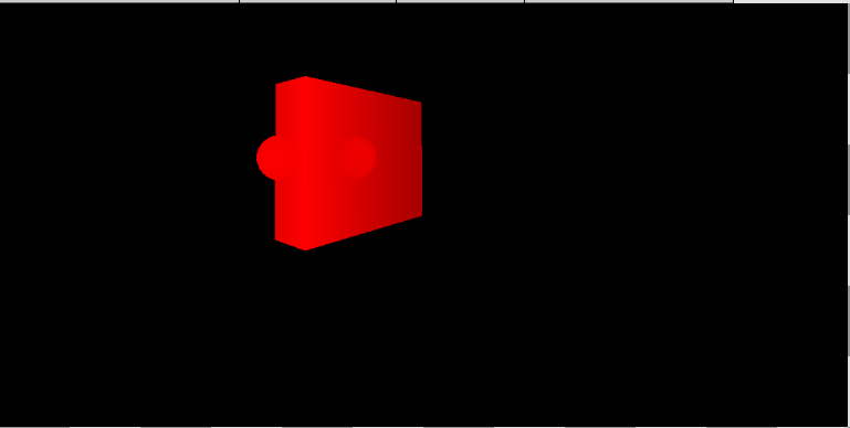
Let’s Render a frame
In this example frame we are going to use a very simple scene. The rectangle is traditional geometry and renders via the traditional deferred path and the spheres are Nanite geometry. Step by step we are going to go through a frame to see what Nanite renders and how it ultimately ends up in the standard G-Buffer. We aren’t going to deal with Shadows and lighting, we’ll do that is part two.
Stage 1 DepthPass
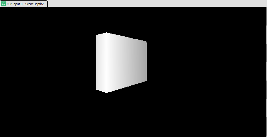
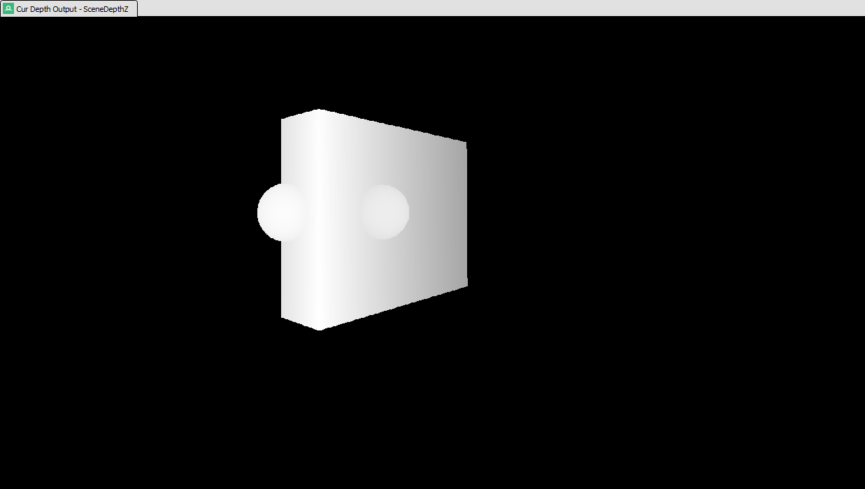
The first stage of rendering is to render the depth of all opaque traditional geometry, this is typically the first pass without Nanite but this is enforced if Nanite is enabled. The main depth buffer in Unreal is called SceneDepthZ and ultimately is the depth buffer used for deferred rendering and all Nanite geometry will ultimately end up in this depth buffer.
Within RenderDoc you can see this is the normal early depth pass
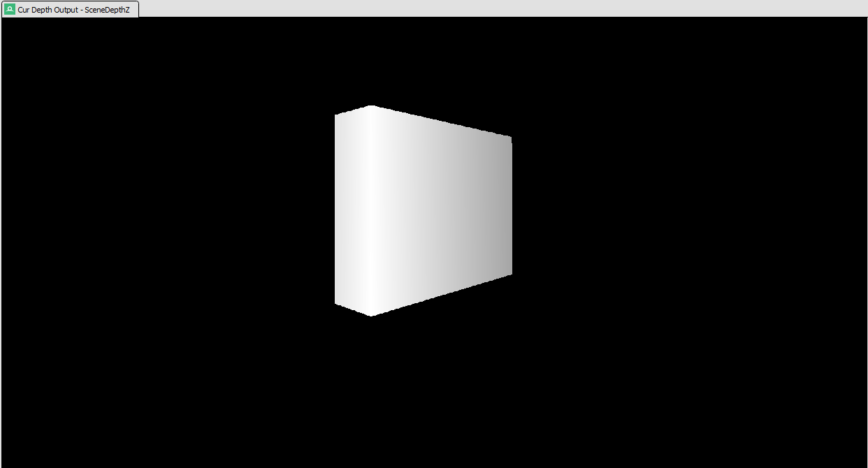
In this simple test scene the only traditional geometry is the rectangle.
Stage 2 InitContext

This one is pretty simple; it’s a compute shader that clears the visibility buffer (VisBuffer64) to default empty values.

Within in editor the allocated size of buffers is bigger than the render size, only the pixels needed for the current window size are rendered. This does not happen in fullscreen builds.
Nanite supports async compute, when enabled this compute based clear of the visibility buffer can overlap with rasterizing of the depth buffer in the previous stage, assuming there are available shader cores.
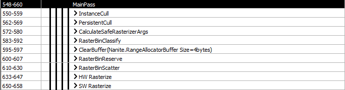
Stage 3 VisBuffer
This is the main render pass for the visibility buffer, everything do to with Nanite rendering is here.
The first thing it does is initialize various queues, remember everything is compute so none of the init can be done on the CPU. InitArgs is a single dispatch of a compute shader that resets all the working buffers that will track clusters across both hardware and software and across main and post passes.
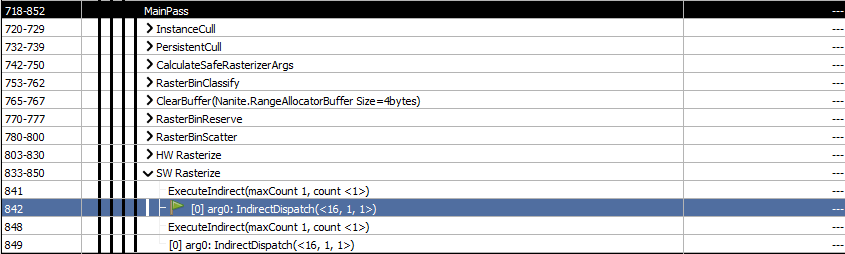
From this point on rendering of the visibility buffer can take one of two forms - it either does one pass of the geometry, or it does two.
This is what two passes looks like, there is a main pass, a HZB build and a post pass. Most frames in a complex scene will do two passes.
When there there is no post pass and Nanite can render everything in a single pass, that single pass is called NoOcclusionPass, it is not called main pass. In RenderDoc it looks slightly different but is equivalent to main pass.

Any nanite pass (main, NoOcclusion or post) breaks down into the following sequence of operations. Although the sequence and theory of the operations is the same in each pass the actual shaders are different due to where it gets data from and what sort of feedback is generated.
Instance Cull - NaniteInstanceCull.usf
This culls whole instances which will be further culled in to clusters in the next step. This step performs frustum culling, distance culling, global plane culling and pixel HZB culling. These individual culling options can be turned on or off with r.Nanite.Culling.Drawdistance, r.Nanite.Culling.Frustum, r.Nanite.Culling.GlobalClipPlane, r.Nanite.Culling.HZB, r.Nanite.Culling.WPODisableDistance.
All nanite data is accessible to the GPU at all times. The static input data to the cull stage is the GPU Scene containing the primitives and the instance data, along with the previous frame HZB texture. Nanite views is an input array of all the views that need to be processed (camera, shadows etc), all active views are processed in a single pass and multiple outputs are produced - we pretty much ignore this for this breakdown.

The output data is all read/write UAV buffers:

Distance culling will cull objects that are too far from the camera and it will also disable WPO in the distance for performance reasons. This WPO disable distance is set by the asset builder on a per instance basis.
HZB culling uses a screen space rect of the instance bounding volume to determine if the whole instance is occluded or not. It tests against the mip map where the screen rect is < 4x4 pixels. The work is done in a shader function called IsVisibleHZB() and GetMinDepthFromHZB(). For the main pass the HZB is the complete previous frame, for the post pass its the HZB that was just generated.
If the instance isn’t visible no further processing is done for the instance, if it is visible (or being forced to render due to various debug flags), then the node is added to the output via function StoreCandidateNode(). The output data actually consists of 2 buffers, one is a byte buffer which contains the actual cluster data (OutMainAndPostNodesAndClusterBatches), the other is OutQueue that contains the atomic state of the output buffer (FQueueState). The node data is 8 bytes per visible instance in the main pass or 12 bytes in the post pass. The first 32bit field is packed with the instance id and node flags, the second 32bit field is view id and the node index. The extra 4 bytes in the post pass data is used to store an enabled bit mask.
InstanceCull also keeps track instances that might be visible but were occluded by the HZB in RWBuffer OutOccludedInstances, the data recorded is the viewid and instanceid.
PersistentCull - NaniteClusterCulling.usf
Most of the culling magic is here…. At a high level this stages processes all the visible instances from the previous stage and generates two lists of clusters that need to be rendered, one for the hardware renderer and one for the software renderer.
The node and cluster culling is the key to Nanite and is where the automatic LOD comes from and is where the concept of virtual geometry comes from. The previous stage culled only instances which are always in memory, this stage culls down to the individual clusters within an instance. The low resolution parent nodes and clusters are always in memory so there is always something that can be rendered. The higher resolution children nodes and clusters may not be in memory. The loading of these higher resolution children is done by the CPU using feedback data from this pass.
All the Nanite cluster data is in a huge virtual byte buffer called Nanite.StreamingManager.ClusterPageData while the BVH hierarchy is in a buffer called Nanite.StreamingManager.Hierarchy. These are both dynamically streamed.
The culling operations that are performed on nodes and clusters are the same as the culling of instances. Backwards facing culling is not performed as most clusters that are facing away from the camera are occlusion culled by the other side of the object. If a parent node is culled and isn’t visible then its children aren’t visible and the processing of that node stops. If a parent node has a small enough triangle size then processing of children stops - this is where the dynamic and automatic LOD comes from. Finally if the memory for a child node isn’t present processing will stop at the parent node and a request will be made for the child - visibly you’ll see a lowe resolution LOD until the higher resolution data is loaded.
A function called PersistentNodeAndClusterCull() in NaniteHierarchyTraversal.ush is responsible for the recursive culling and traversal of the per-mesh node and cluster BVHs. Tree-culling in a compute shader is awkward as the number of nodes that need to be processed is dynamic and can be anywhere from zero to hundreds of thousands, the CPU would need to know up front what to dispatch. Mapping compute threads 1:1 to trees can result in extremely long serial processing that severely under utilizes the GPU and takes too long. Conversely, mapping threads 1:1 to leaf nodes can end up leaving most threads idle.
For optimal GPU processing the CPU spawns just enough worker threads to fill the GPU and uses a Multiple Producer, Multiple Consumer job queue to keep the threads busy. A worker thread atomically consumes the next item in the queue and keeps going until there is nothing left. The work queue can contain nodes or cluster and initially the queue is populated with only nodes generated by preceding instance cull pass Workers threads will continuously consume items from the queue and sometimes produce new items which are atomically added to the end. When nodes are processed they will append work items to the queue for each of the visible children, this work will be in the form of a new node, or if at a leaf a cluster of triangles. Once the queue is empty all the work is done. The two core functions that do the work are ProcessNodeBatch and ProcessClusterBatch. Only nodes generate new work, clusters are only consumed and never generate new work.
Once the culling process stops the initial set of instances that might represent billions of triangles have been hierarchically reduced to just what is visible, and those visible clusters have a fairly consistent number of triangles per frame because LOD for a given cluster automatically happens based on screen error. .
This stage can appear as
NodeAndClusterCullin a capture, the difference isPersistentCullis a single kernel that operates on an atomic list of nodes and clusters, whereasNodeAndClusterCullis multiple compute kernels that operate either on nodes or clusters.PersistentCullis the current default as it is more efficient.GNanitePersistentThreadCullingis used to select between them in code and this is controlled byr.Nanite.PersistentThreadCulling
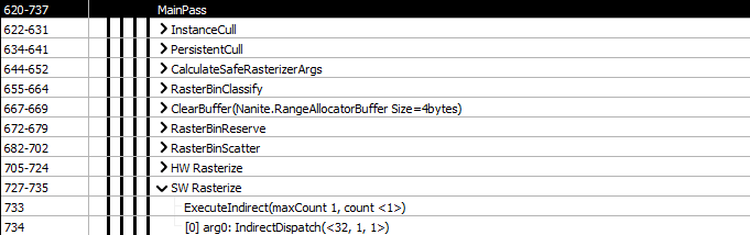
CalculateSafeRasterizerArgs, RasterBinClassify, RasterBinReserve, RasterBinScatter
These next 4 compute stages are grouped together, all of them are in NaniteRasterBinning.usf.
These stages ultimately generate the execute indirect buffers and the draw indirect buffers for the following software and hardware render stages. Remember there is no CPU involvement so even the most simple tasks are done as multiple passes in compute.
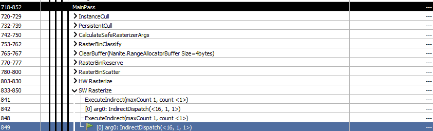
HW Rasterize, SW Rasterize
HW Rasterize uses a traditional pixel shader to render large triangle clusters to the visibility buffer, while SW Rasterize uses a compute shader to render small triangle clusters to the same visibility buffer. The reason it is possible to mix hardware and software rendering without issues such as depth fighting or cracks along edges of triangles, is because DX12 has super strict and very well-defined rasterization rules. The software rasterizer can replicate these rules and seamlessly interact with the hardware renderer so triangles can touch or intersect without any cracks or discontinuities.
As previously stated HW rasterize is better suited to large triangles, SW for very small triangles. The split between HW and SW is performed by PersisentCull based on the projected screen area of the cluster - it doesn’t know anything about the size of the triangles within the cluster so artists should keep them consistent when building meshes.
The visibility buffer has fixed data for the hardware and software renders, and this data is independent of the materials, therefore shaders don’t have to changes and everything can be rendered by a single draw and/or compute call. World position offset on a material does change the vertex processing which does require shader changes, for the compute path this is an entirely new monolithic shader. Every WPO material will require its own shaders and its own set of draw calls.
Async compute can allow the software rasterizer to run at the same time as the hardware rasterizer. It is controlled in code by r.Nanite.AsyncRasterization but the GPU also has to support async compute (GSupportsEfficientAsyncCompute is true). On DX12 nvidia hardware does not support compatible async compute but AMD does. Xbox and PS5 always sets GSupportsEfficientAsyncCompute and is a good reason to test on AMD hardware and Xbox/PS5.
For performance comparison, all clusters can be forced to the hardware rasterizer by setting r.Nanite.ComputeRasterization 0. You can’t force everything to render with software.
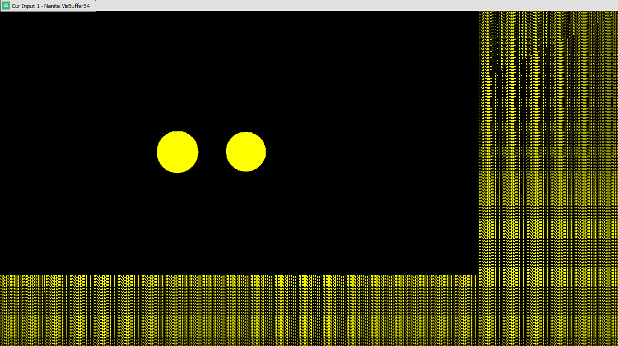
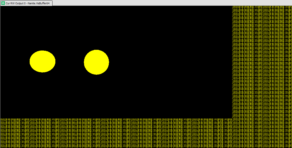
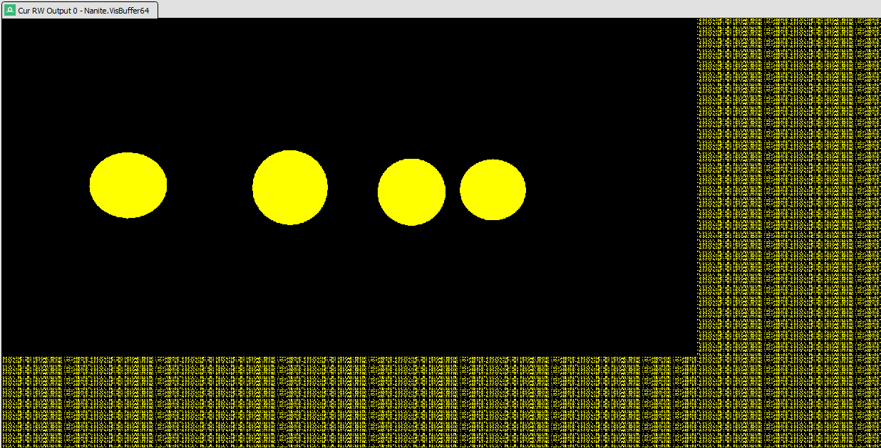
For our simple test scene this is the resulting visibility buffer, in this case rendered entirely by the software rasterizer in a single pass.
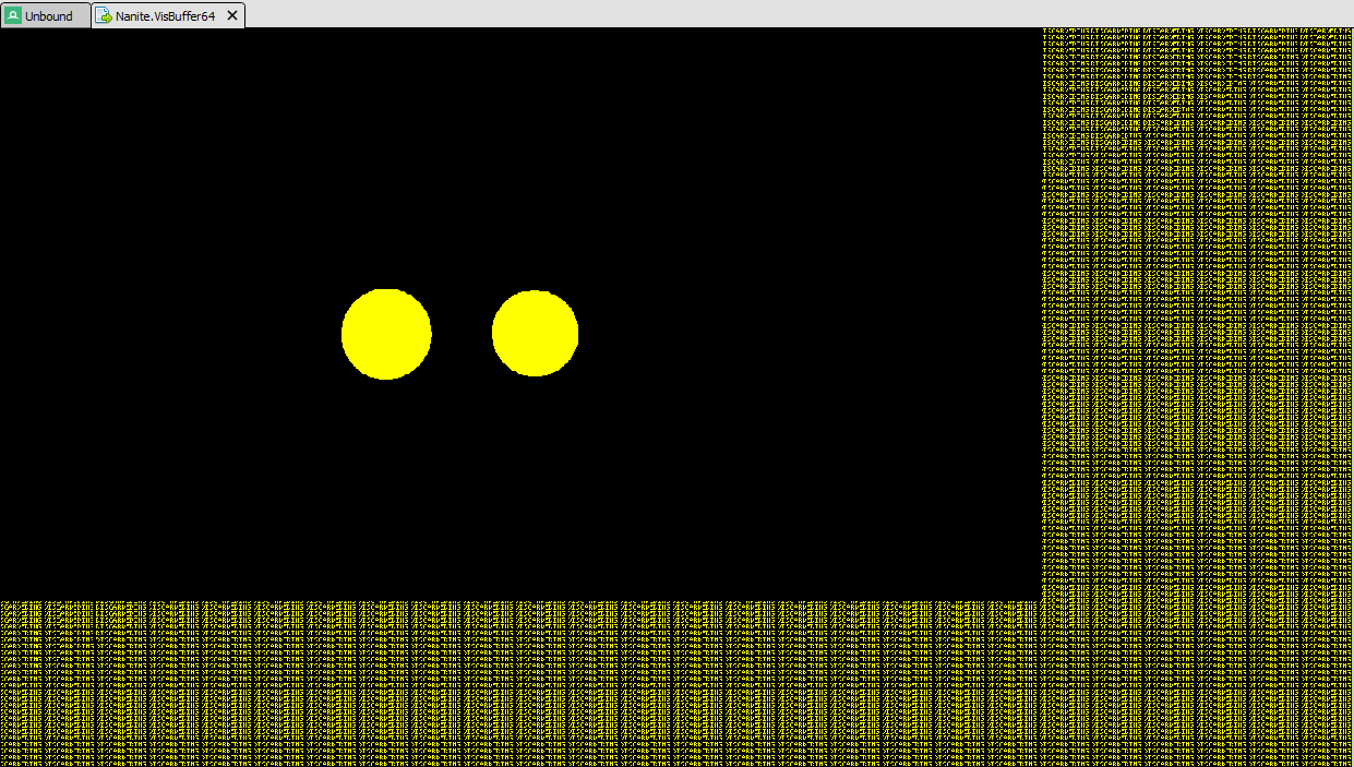 The visibility buffer contains just Nanite geometry, there is no interaction at this point with Nanite and traditional geometry.
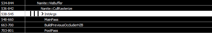
BuildPreviousOccluderHZB
This stage is only present if there is a post pass and takes in SceneDepthZ (the traditional depth buffer) along with the current and up to date Nanite visibility buffer and it generates a new HZB that will be used by the post pass. It does this by using 3 consecutive compute shaders:
The first pass takes the current Nanite visibility buffer, which also contains Nanite depth, and the traditional depth buffer, combines the depths and generates the first three mips of the new HZB. The polygon data in the visibility buffer isn’t needed at this stage.
The tranditional depth buffer contents
The visibility buffer contents including 32bits of depth
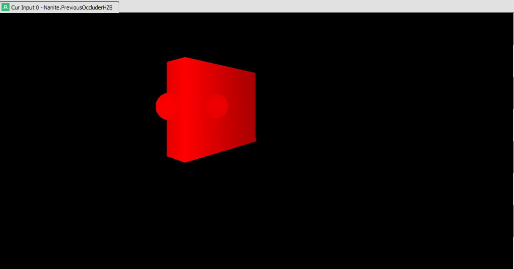
The output includes all Nanite and traditional geometry. This is the highest resolution buffer in the stack, final two compute shaders take this and generate lower mips.
Stage4 EmitDepthTargets
At this stage the main and post pass are done and rendering of the visibility buffer is complete. This is where the visibility buffer starts to be resolved in to the standard G Buffer. Everything from here is a screen space operation.
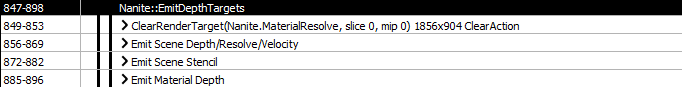
ClearRenderTarget
This one is pretty self explanatory. Nanite.MaterialResolve is a 2 channel frame buffer that holds the global material ID and various flags for each visible Nanite pixel, before running the material resolve the material id buffer is cleared to black. Within this 2 channel 32bit integer frame buffer, R contains material info flags like receives decals, has distance fields, shading bin and lighting channels - basically things needed later. G is the material id, in our example the material id is zero as there is only one material.
The function PackMaterialResolve() packs all the required data into the pair of 32bit values.
Emit Scene Depth/Resolve/Velocity (NaniteExportGBuffer.usf)
The material resolve computes the triangle and material information from the Nanite visibility buffer. The material id is only written if the Nanite depth is in front of the scene depth and the scene depth is updated. This is where Nanite depth gets combined with the main depth buffer, Nanite pixels that are in front will use depth write in the pixel shader to update SceneDepthZ. The result is a complete depth buffer and a material id buffer containing only the visible Nanite pixels, Nanite pixels behind traditional geometry have now been culled on a per pixel level, any Nanite clusters that incorrectly passed through HZB culling are now correctly resolved.
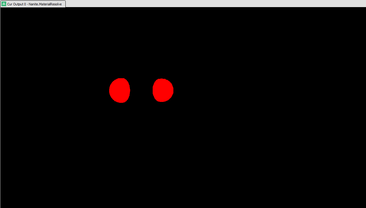
Nanite.MaterialResolve contains flags in the red channel and the material ID in the green channel. This shader also processes the depth buffer, for the first time we have just the visible Nanite pixels with respect to the traditional depth buffer. These are the only pixels that will be processed going forwards.
SceneDepthZ is now complete and can be used for traditional deferred shading and computing world space positions without regard for which pixels are Nanite.
The same shader writes pixel velocity but only for transform based movement - either the object moving or the camera moving, pixel velocity from WPO movement is evaluated later (another reason why WPO on nanite is slower)
Emit Scene Stencil
This is only present if the pixel shader hardware cannot write stencil reference values from the shader. If the hardware can write stencil values then this pass is combined with the prior.
The stencil is written based on flags in the material, it is used for things like decal materials.
Emit Material Depth
This stage converts the material ID to a hardware depth buffer. This sounds weird but its one of the very clever features of Nanite. Later on we are going to have to identify materials based on the material ID value, the GPU already has hardware to efficiently mass reject or accept pixels based on a value - its called the depth compare. If the material ID is in a pixel buffer then every material shader will have to do a texture read and compare at the top of the shader and terminate if the material is the wrong ID, If a depth buffer is prepared where each material has a different depth value, the depth compare hardware can be used to cull/accept pixels before the pixel shader even runs!! This is genius.
The input is Nanite.MaterialResolve and the output looks like this:
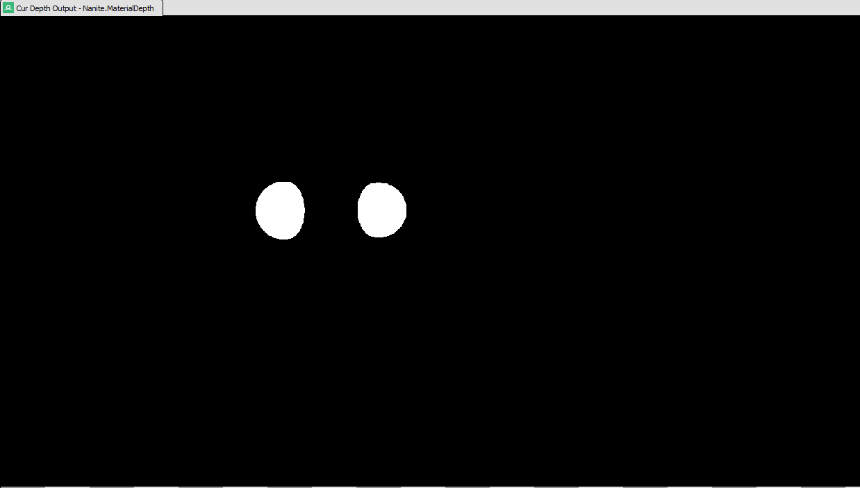
Our simple test scene only has a single Nanite material so for this example all the white pixels are the same value (real depth=0.00006)
Stage5 BasePass
Before the Nanite base pass is performed the base pass is performed on traditional geometry
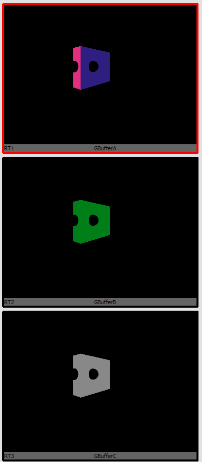
The traditional geometry pixels are now in the G-Buffer via the completely normal render path. The only interaction with Nanite at this point is that traditional pixels aren’t processed where Nanite pixels will ultimately be.
Nanite materials are added on top of this with a full screen pass per material using the nanite material depth buffer.
This can become a performance problem as every Nanite material has to do a full screen pass, this operation can get very expensive at high resolutions. Remember everything is running on GPU so there a few compute shaders that execute prior to this to generate indirect draw buffers, these compute shaders also cull materials that aren’t visible so we aren’t don’t a full screen pass for every material in the world.

In our case we only have one nanite material so there is only a single draw
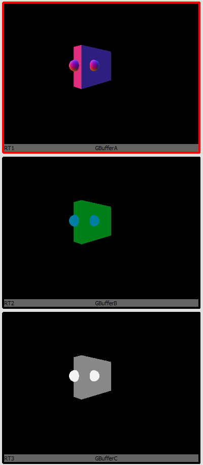
The pixel shader used for the fullscreen material pass is compiled from the material graph editor and is generated in much the same way as any other materials pixel shader. It is in these Nanite pixel shaders that the visibility buffer is resolved and all the pixel gradients are computed.
From this point on Nanite geometry is in the G-Buffer and identical to any other geometry as far as future lighting and shadows are concerned.
Multiple Nanite Materials
Lets make a new scene with 3 materials across 4 spheres. The two black spheres have the same material, the blue and white are different materials, all are Nanite meshes.
All the Nantie geometry is rendered in a single API call, because the visibility buffer is independent of material, in this example everything is rendered by SW Rasterize.
However now we have three different materials and the Nanite.MaterialResolve shows this. The two red spheres have the same material ID of zero, whereas the two yellow spheres are different, one has a material ID of 1 and the other 2.
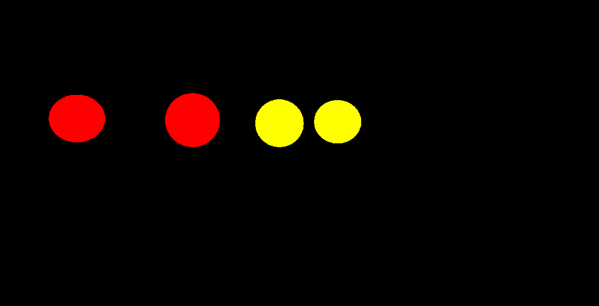
This is pretty much what you would expect from what we know about how Nanite resolves materials.
The material depth buffer is also what you would expect
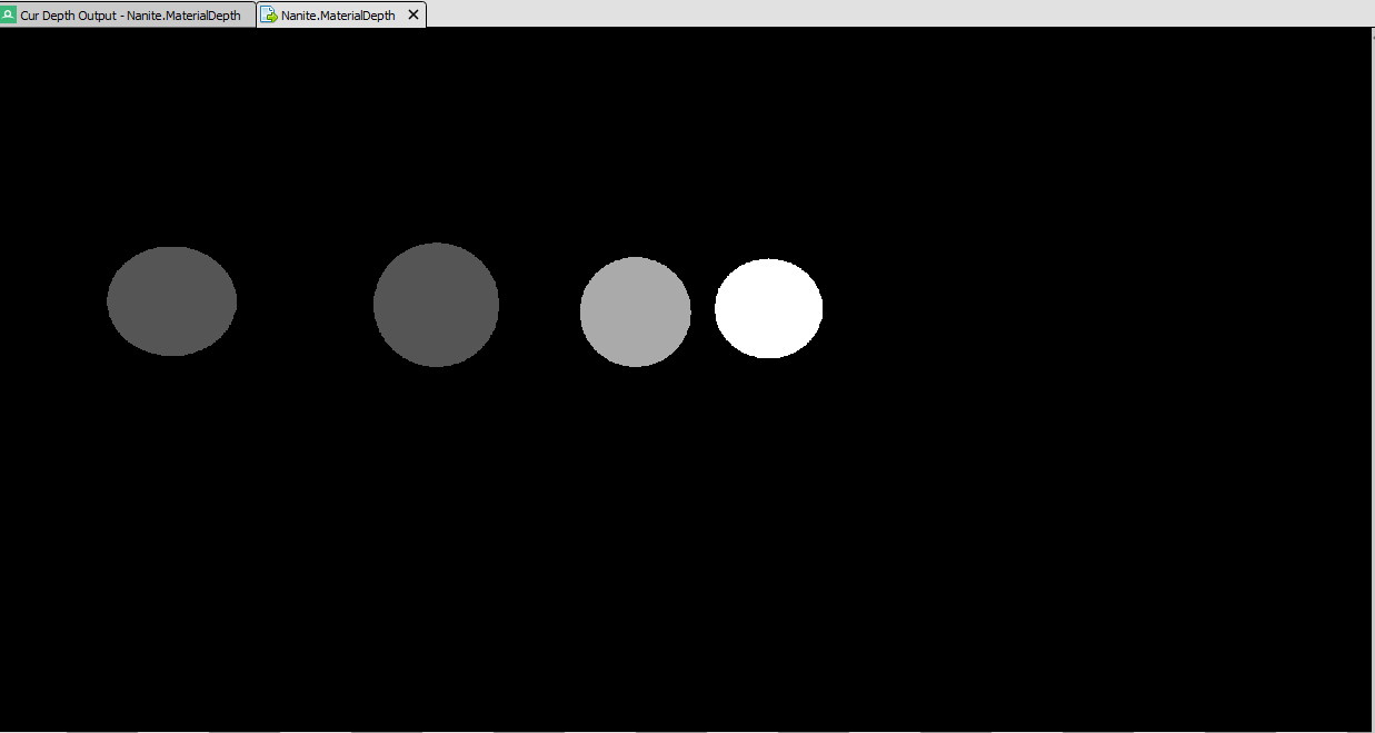
The depth values are 0.00006, 0.00012 and 0.00018 for the three materials.
Up to here nothing is really any different regardless of the number of materials used in the scene. The base pass is where things are different, there is indeed one full-screen quad rendered per material.
These full-screen passes take about 20uS as a given material is only evaluated for pixels that use that material due to the depth test trick using the Material Depth buffer. In reality there needs to be a lot of expensive materials covering a lot of pixels for this stage to really be expensive but can happen.
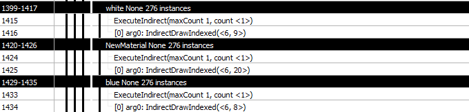
There is indeed a full screen pass per material
WPO Materials
Let’s take the above scene and add a simple WPO calculation to the black material (left two spheres).
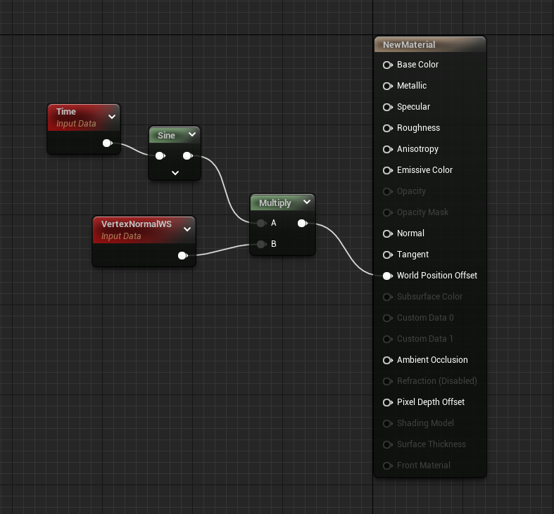
Once WPO is enabled on a Nanite mesh it is important to set the Max displacement in the material details panel. Any displacement above this amount is clamped. This is quite important for Nanite is its used to create maximum extent nodes that can be safely culled.

You only need to specify this value if the WPO can make the object bigger, if it stays within its original bounds this value does not need to be set. Leaving this value at 0.0 disables clamping, any WPO offset is allowed, but it won’t modify any bounding volumes - incorrect culling and flickering can result.
None Nanite materials should set this too.
The Nanite software renderer is a monolithic compute shader that does all the vertex processing, rasterization and pixel processing. For a non WPO material that vertex and pixel processing is always the same, hence why we can use a single draw for all materials. However, when WPO is enabled the vertex pipeline needs to be modified, the final position is no longer a simple transform but the result of the material graph. The base vertex code used by the HW vertex shaders and the SW compute shaders is NaniteVertexFactory.usf and this uses a function called GetMaterialWorldPositionOffset() which is by default an empty function. When you create a WPO material, the code required for the WPO operation is injected in to GetMaterialWorldPositionOffset() and a new set of shaders is generated.
The WPO operation implemented in GetMaterialWorldPositionOffset() is called multiple times in the vertex factory because it needs velocity which means WPO is computed for this frame and last frame. Unlike the traditional renderer where velocity can be computed in the vertex shader and and passed to the pixel shader, Nanite must compute the velocity at each pixel which means the entire WPO graph has to be evaluated twice. The early velocity buffer cannot be used by WPO materials for local movement, final velocity is always computed at each pixel with the velocity buffer being combined with the local WPO velocity. Any WPO on Nanite should be a very simple function because of the number of evaluations.
For Nanite every different WPO material will be a different draw call.
The first dispatch draws both the WPO objects in SW, yes multiple objects with the same material will draw at once. This is using the custom generated WPO SW Rasterize compute shader.
The second dispatch draws the non WPO objects with the default nanite compute shader.
If we force HW rasterizing once again we still have 2 render passes, one for the WPO material and one for the none WPO material. For the HW path WPO generates a new pixel shader and vertex shader.
Fallback Mesh
Every Nanite mesh has a fallback mesh used for per poly collision, UV unwrapping, light baking, ray tracing etc. The fallback mesh is also used for rendering if nanite is disabled or not supported - this may be important for DX11 if that is the minimum spec PC.
On platforms that do support Nanite you can disable Nanite globally with r.Nanite 0 and force all the fallback meshes to render, r.Nanite.ProxyRenderMode 0 means render the fallback mesh if Nanite is not available, r.Nanite.ProxyRenderMode 1 means don’t render nanite at all.
In the mesh editor there are options for specifying the resolution and quality of the fallback mesh, along with the ability to specify a custom fallback mesh/LODs. In a game that only runs on platforms that support Nanite a large memory saving can be had by setting the fallback mesh to be very low resolution or potentially nonexistent if none of the CPU side features are needed or data is supplied in other ways such as custom collision meshes.
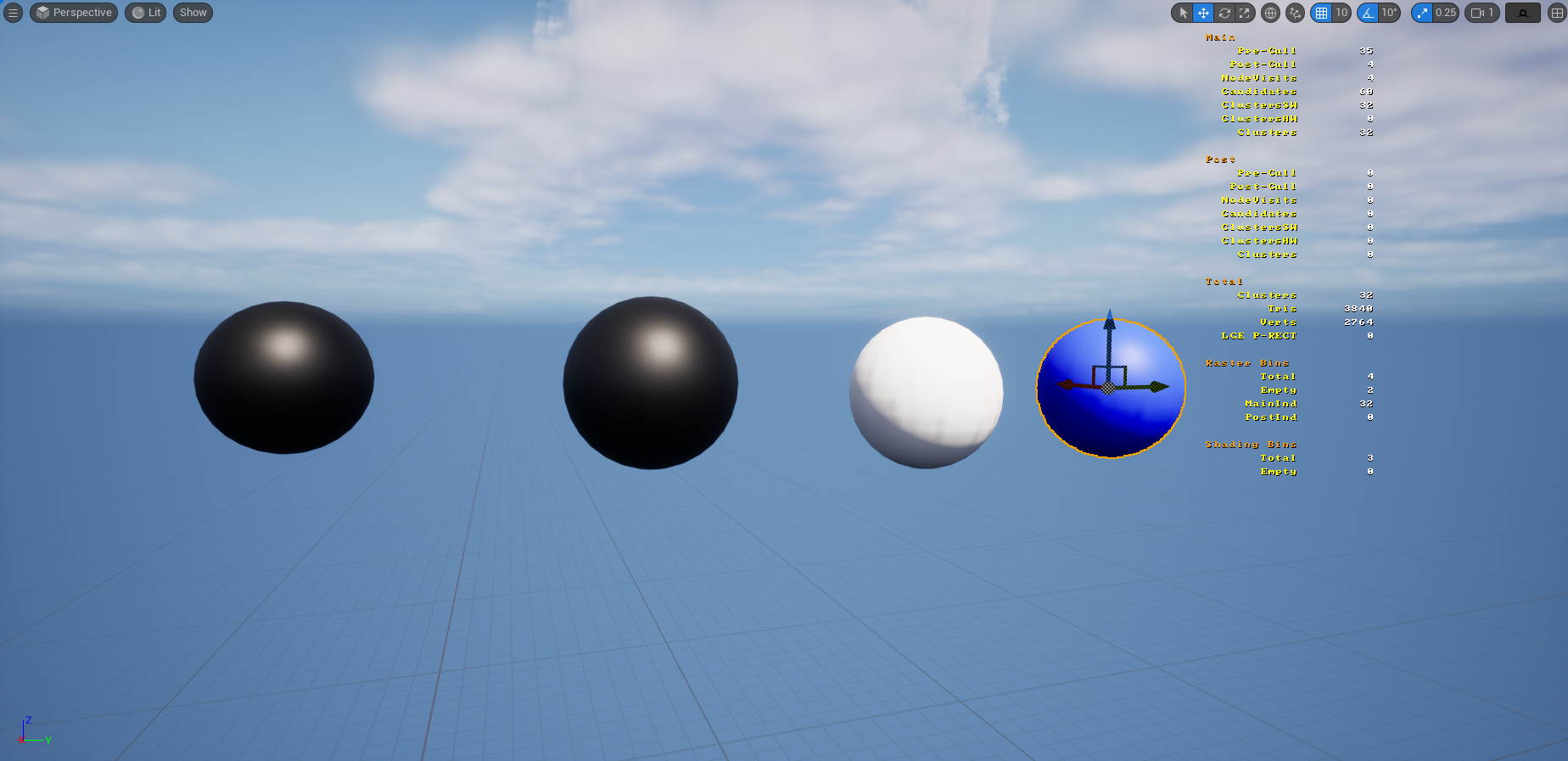
Nanite Stats
What do the primary Nanite stats mean and what are we looking for?
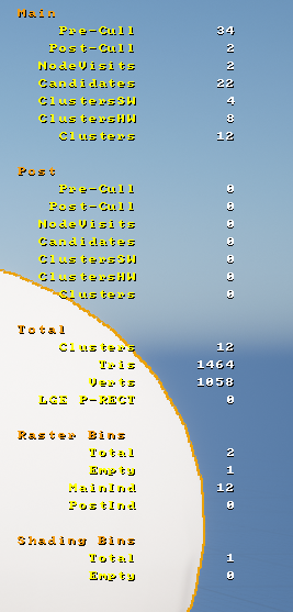
main and post refer to the two Nanite passes, the stats within the two blocks are the same. The main pass is the first pass that uses last frames HZB, the post pass is the geometry that wasn’t rendered last frame or its simply unsure about it. Ideally you want most geometry in the main pass.
pre-cull is the number of instances before culling
post-cull is the number of instances after the instance culling stage - visibile or partially visible instances.
The number of instances isn’t really a factor because they further broken down in to clusters. However, having uniform shapes that are easy to bound in a sphere or a screen space rectangle will help with rejecting instances.
Node visits is the number of BVH nodes that were visited (part of the second stage culling in NodeAndClusterCulling). This will at least be the number of instances because every instance has at least one BVH node. You don’t have much control over this because the BVH for an instance is built for you.
candidates this is the number of candidate render clusters prior to cluster culling.
ClustersSW The number of clusters rendered by the software compute path. Keeping triangles within a cluster a consistent size will make the cluster render quicker.
ClustersHW The number of clusters rendered by the hardware rasterizer (traditional GPU). Lots of clusters in here indicate large triangles that aren’t ideal for Nanite.
Clusters The total number of clusters rendered via any path
The total section is the sum of the main and post passes.
Clusters is the total number of clusters in the entire frame (summed across the 4 passes, HW+SW from main and post).
Tris total number of triangles in the rendered clusters
Verts total number of verts in the rendered clusters.
Nanite Overview visualizer
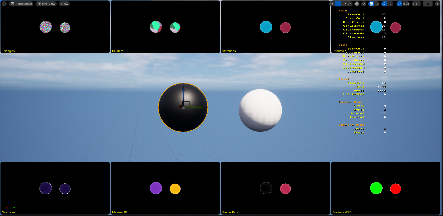
A lot of these are self explanatory.
Evaluate WPO This shows what materials use WPO. Green has WPO, red doesn’t. You want lots of red here. If there is green make sure they use a minimal number of WPO materials so you aren’t switching shaders all the time.
Material ID show the total number of Nanite materials. Remember Nanite performs a full screen pass for every material, there every different color in this view is a full screen pass to lay down the G-Buffer. Use this with the Evaluate WPO view to see how many WPO materials are being used.
Raster bins is how the scene was grouped in to bins which represent batches of geometry. It could be a single bin but is typically 4, one for each of HW+SW in main and post passes. WPO will seriously mess this up especially if there are lots of WPO materials.
Overdraw This is a big one to check when looking for performance problems. Nanite only supports opaque geometry so in theory it should all nicely occlude and there should be minimal overdraw. This is mostly true but Nanite supports masked alpha which messes with the culling and it’s possible to make geometry that is difficult to cull. Remember it is clusters that are culled in the HZB not triangles therefore if any part of the cluster is visible the entire 128 triangle cluster is rendered. This makes things like foliage very difficult to cluster cull and you’ll see the overdraw and the number of rendered clusters go through the roof. Why is foliage problematic to render? First of all, it’s difficult to make 128 triangle clusters that have nice shape when projected into screen space - this makes getting false positives for visibility really easy. Second, it’s easy to get to holes in the depth buffer where a single pixel of the back plane or distant geometry is visible, these depth holes, even one pixel in size, push the HZB back to the farthest visible distance. When the mips of the HZB are generated, the output pixel is the furthest of all the input pixels, this makes the small HZB levels almost useless for culling as the farthest distance in any HZB pixel is the distant geometry or back plane.
Debug Rendering
Nanite has a lot of debug modes and visualizers in the editor. Some of the debug features force shaders to output to multiple frame buffers when they technically don’t need to. Any profiling should be done in a full retail build where these features will be disabled.